Drifters module - demo

pynsitu.drifters implements methods useful to the cleaning and processing of drifter trajectories.

Drifter data is assumed to be contained within a pandas dataframe with with a least the following columns: time, longitude, latitude. A column may also described the drifter id.

import xarray as xr
import pandas as pd
import numpy as np

import matplotlib.pyplot as plt

import pynsitu as pin

---

generate synthetic drifter trajectories

def generate_one_trajectory(
    u_mean=-0.1, v_mean=0, u_wave=0.1, noise=0.05, dr_id="dr0", end="2018-02-01"
):

    freq = "1H"

    time_unit = pd.Timedelta("1s")
    dt = pd.Timedelta(freq) / time_unit
    time = pd.date_range(start="2018-01-01", end=end, freq=freq)
    _time = (time - time[0]) / time_unit

    lon0, lat0 = -20, 30
    scale_lat = 111e3
    scale_lon = scale_lat * np.cos(lat0 * pin.deg2rad)
    T = pd.Timedelta("1D") / time_unit

    u = (
        u_mean
        + u_wave * np.cos(2 * np.pi * _time / T)
        + np.random.randn(time.size) * noise
    )
    v = (
        v_mean
        + u_wave * np.sin(2 * np.pi * _time / T)
        + np.random.randn(time.size) * noise
    )

    lon = lon0 + np.cumsum(u) * dt / scale_lon
    lat = lat0 + np.cumsum(v) * dt / scale_lat
    # lon = u
    # lat = v

    df = pd.DataFrame(dict(lon=lon, lat=lat, time=time, u=u, v=v))
    df["id"] = dr_id
    df = df.set_index("time")

    return df

# actually generate one time series
df = generate_one_trajectory()
df.head()

	lon	lat	u	v	id
time
2018-01-01 00:00:00	-20.000788	29.999491	-0.021034	-0.015686	dr0
2018-01-01 01:00:00	-20.001118	29.998477	-0.008826	-0.031258	dr0
2018-01-01 02:00:00	-19.997529	29.999040	0.095854	0.017331	dr0
2018-01-01 03:00:00	-20.000823	30.002137	-0.087982	0.095500	dr0
2018-01-01 04:00:00	-20.004857	30.005824	-0.107715	0.113700	dr0

---

basic plots to inspect data

May be useful to clean up drifter time series

df.geo.plot_bokeh()

Loading BokehJS ...

phv, coords = df.geo.plot_on_map()
phv

compute velocities

Multiple methods are employed to compute velocities, see compute_velocities doc and code. Some involve projecting data which results in local cartesian coordinates x and y.

df.geo.compute_velocities(inplace=True)
df.head()

	lon	lat	u	v	id	x	y	velocity_east	velocity_north	velocity
time
2018-01-01 00:00:00	-20.000788	29.999491	-0.021034	-0.015686	dr0	133960.361743	1031.830412	-0.113929	-0.079742	0.139063
2018-01-01 01:00:00	-20.001118	29.998477	-0.008826	-0.031258	dr0	133929.833767	919.064918	0.043676	-0.006953	0.044226
2018-01-01 02:00:00	-19.997529	29.999040	0.095854	0.017331	dr0	134275.412685	985.574663	0.003952	0.056342	0.056480
2018-01-01 03:00:00	-20.000823	30.002137	-0.087982	0.095500	dr0	133953.359341	1325.061218	-0.098208	0.104462	0.143378
2018-01-01 04:00:00	-20.004857	30.005824	-0.107715	0.113700	dr0	133559.241127	1729.127419	-0.115983	0.087820	0.145480

df.geo.plot_bokeh(velocity=True)

Loading BokehJS ...

phv, coords = df.geo.plot_on_map(s=10, c="velocity", clim=(0, 0.3), cmap="magma")
phv

compare different methods to compute velocities

df_sp = df.geo.compute_velocities(distance="spectral", inplace=False)
df_xy = df.geo.compute_velocities(distance="xy", inplace=False)

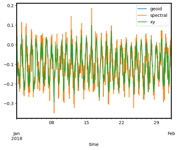
df["velocity_east"].plot(label="geoid")
df_sp["velocity_east"].plot(label="spectral")
df_xy["velocity_east"].plot(label="xy")
plt.legend()

<matplotlib.legend.Legend at 0x1367f8cd0>

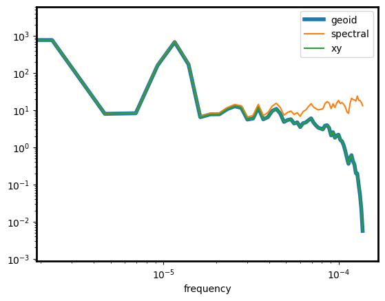
kwargs = dict(include=["velocity_east"], nperseg=24 * 5, detrend=False)
E = df.ts.spectrum(**kwargs)
E_sp = df_sp.ts.spectrum(**kwargs)
E_xy = df_xy.ts.spectrum(**kwargs)

# spectrum comparison
ax = E["velocity_east"].rename("geoid").plot(lw=4)
E_sp["velocity_east"].rename("spectral").plot(ax=ax)
E_xy["velocity_east"].rename("xy").plot(ax=ax)
ax.set_yscale("log")
ax.set_xscale("log")
ax.legend()

<matplotlib.legend.Legend at 0x136bca170>

---

concatenate multiple trajectories and manipulate

ids = [0, 1, 2]
u_wave = [0, 0.1, 0.2]
dfm = (
    pd.concat(
        [
            generate_one_trajectory(
                u_mean=-0.1, v_mean=0, u_wave=uw, noise=0.05, dr_id=f"dr{i}"
            )
            for i, uw in zip(ids, u_wave)
        ]
    )
    .reset_index()
    .set_index("id")
)

# get all drifter ids
ids = list(dfm.index.unique())

dfm.head()

	time	lon	lat	u	v
id
dr0	2018-01-01 00:00:00	-20.001938	30.001574	-0.051755	0.048540
dr0	2018-01-01 01:00:00	-20.003740	29.999217	-0.048114	-0.072674
dr0	2018-01-01 02:00:00	-20.007893	29.998033	-0.110882	-0.036504
dr0	2018-01-01 03:00:00	-20.014289	29.997121	-0.170800	-0.028130
dr0	2018-01-01 04:00:00	-20.018838	29.996461	-0.121469	-0.020351

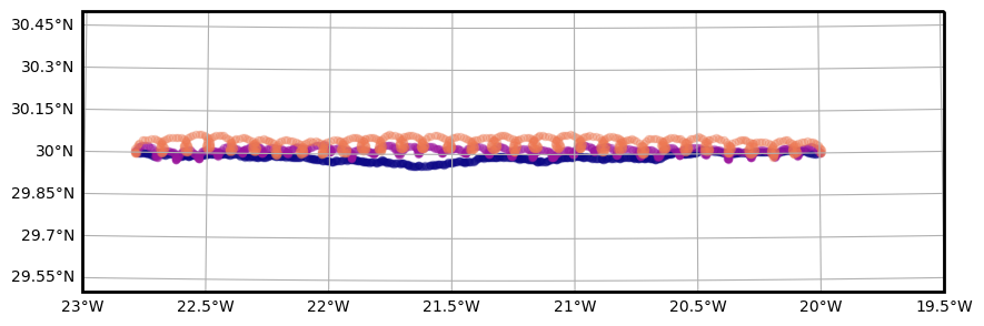
fig, ax, _ = pin.maps.plot_map(extent=[-23.0, -19.5, 29.5, 30.5])

colors = pin.get_cmap_colors(len(ids))

for i, c in zip(ids, colors):
    dfm.loc[i].plot.scatter(
        ax=ax, x="lon", y="lat", c=c, alpha=0.3, transform=pin.maps.crs
    )

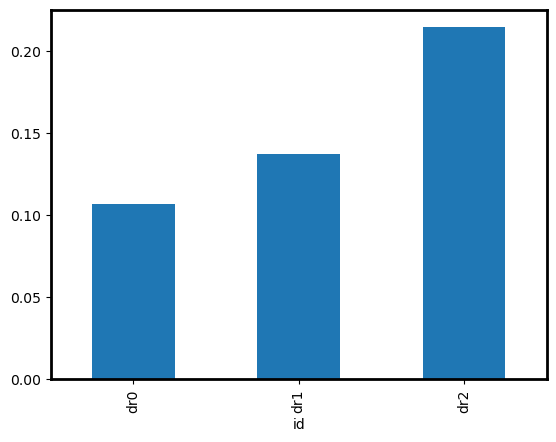
Compute velocities and averaged energy per drifter

dfm_vel = (
    dfm.groupby("id")
    .apply(lambda df: df.set_index("time").geo.compute_velocities().reset_index())
    .droplevel(1)
)

dfm_vel.groupby("id")["velocity"].mean().plot.bar()

<Axes: xlabel='id'>

---

compute temporal window averaged diagnostics (spectra, autocorrelations)

When manipulating drifter time series one may need to divide the timeseries into chunks (“windows”) and performs diagnostics on each chunk separately before combining results. This may typically be the case for spectral or autocorrelation diagnostics.

df = generate_one_trajectory(dr_id="dr0", end="2018-04-01")

def compute_periodogram(df, **kwargs):
    df["U"] = df["u"] + 1j * df["v"]
    return df.ts.spectrum(method="periodogram", unit="1D", include=["U"], **kwargs)["U"]


P = pin.drifters.time_window_processing(
    df,
    compute_periodogram,
    "10D",
    geo=True,
    detrend="linear",
)
P = P.reset_index()

# assembles as an xarray dataset
coords = ["time", "lon", "lat", "id"]
P_stacked = (
    P.drop(columns=coords)
    .stack()
    .to_xarray()
    .rename(level_0="index", level_1="frequency")
    .rename("uv")
)
P_stacked["frequency"] = P_stacked["frequency"].astype(float)
P_xr = xr.merge(
    [
        P[coords].to_xarray(),
        P_stacked,
    ]
)
P_xr

<xarray.Dataset>
Dimensions:    (index: 16, frequency: 2161)
Coordinates:
  * index      (index) int64 0 1 2 3 4 5 6 7 8 9 10 11 12 13 14 15
  * frequency  (frequency) float64 -11.99 -11.98 -11.97 ... 11.97 11.98 11.99
Data variables:
    time       (index) datetime64[ns] 2018-01-06 2018-01-11 ... 2018-03-22
    lon        (index) float64 -20.5 -20.95 -21.39 ... -26.25 -26.7 -27.13
    lat        (index) float64 29.99 29.97 29.96 29.94 ... 29.86 29.86 29.87
    id         (index) object 'dr0' 'dr0' 'dr0' 'dr0' ... 'dr0' 'dr0' 'dr0'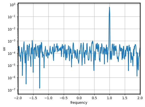
    uv         (index, frequency) float64 0.0002499 5.11e-05 ... 0.0003054

xarray.Dataset

• Dimensions:
  • index: 16
  • frequency: 2161
• Coordinates: (2)
  • index
    (index)
    int64
    0 1 2 3 4 5 6 ... 10 11 12 13 14 15

    array([ 0,  1,  2,  3,  4,  5,  6,  7,  8,  9, 10, 11, 12, 13, 14, 15])

  • frequency
    (frequency)
    float64
    -11.99 -11.98 ... 11.98 11.99

    array([-11.994447, -11.983341, -11.972235, ...,  11.972235,  11.983341,
            11.994447])

• Data variables: (5)
  • time
    (index)
    datetime64[ns]
    2018-01-06 ... 2018-03-22

    array(['2018-01-06T00:00:00.000000000', '2018-01-11T00:00:00.000000000',
           '2018-01-16T00:00:00.000000000', '2018-01-21T00:00:00.000000000',
           '2018-01-26T00:00:00.000000000', '2018-01-31T00:00:00.000000000',
           '2018-02-05T00:00:00.000000000', '2018-02-10T00:00:00.000000000',
           '2018-02-15T00:00:00.000000000', '2018-02-20T00:00:00.000000000',
           '2018-02-25T00:00:00.000000000', '2018-03-02T00:00:00.000000000',
           '2018-03-07T00:00:00.000000000', '2018-03-12T00:00:00.000000000',
           '2018-03-17T00:00:00.000000000', '2018-03-22T00:00:00.000000000'],
          dtype='datetime64[ns]')

  • lon
    (index)
    float64
    -20.5 -20.95 ... -26.7 -27.13

    array([-20.50148473, -20.95427095, -21.38775437, -21.81710021,
           -22.24394721, -22.68268247, -23.11610552, -23.56039701,
           -24.02126706, -24.46964428, -24.91225274, -25.35694082,
           -25.8024769 , -26.25201327, -26.69832579, -27.13053615])

  • lat
    (index)
    float64
    29.99 29.97 29.96 ... 29.86 29.87

    array([29.98733161, 29.97104511, 29.95834349, 29.94076669, 29.92065464,
           29.90709828, 29.90559696, 29.9101361 , 29.90207877, 29.89100958,
           29.89347973, 29.88774745, 29.87169467, 29.86424073, 29.86305365,
           29.87362302])

  • id
    (index)
    object
    'dr0' 'dr0' 'dr0' ... 'dr0' 'dr0'

    array(['dr0', 'dr0', 'dr0', 'dr0', 'dr0', 'dr0', 'dr0', 'dr0', 'dr0',
           'dr0', 'dr0', 'dr0', 'dr0', 'dr0', 'dr0', 'dr0'], dtype=object)

  • uv
    (index, frequency)
    float64
    0.0002499 5.11e-05 ... 0.0003054

    array([[2.49860506e-04, 5.10987585e-05, 1.71218405e-05, ...,
            4.20965337e-04, 4.97755244e-04, 3.05366279e-04],
           [2.49860506e-04, 5.10987585e-05, 1.71218405e-05, ...,
            4.20965337e-04, 4.97755244e-04, 3.05366279e-04],
           [2.49860506e-04, 5.10987585e-05, 1.71218405e-05, ...,
            4.20965337e-04, 4.97755244e-04, 3.05366279e-04],
           ...,
           [2.49860506e-04, 5.10987585e-05, 1.71218405e-05, ...,
            4.20965337e-04, 4.97755244e-04, 3.05366279e-04],
           [2.49860506e-04, 5.10987585e-05, 1.71218405e-05, ...,
            4.20965337e-04, 4.97755244e-04, 3.05366279e-04],
           [2.49860506e-04, 5.10987585e-05, 1.71218405e-05, ...,
            4.20965337e-04, 4.97755244e-04, 3.05366279e-04]])

• Indexes: (2)
  • index
    PandasIndex

    PandasIndex(RangeIndex(start=0, stop=16, step=1, name='index'))

  • frequency
    PandasIndex

    PandasIndex(Index([ -11.99444701527071, -11.983341045812125, -11.972235076353542,
           -11.961129106894958, -11.950023137436373,  -11.93891716797779,
           -11.927811198519207, -11.916705229060621, -11.905599259602038,
           -11.894493290143453,
           ...
            11.894493290143453,  11.905599259602038,  11.916705229060621,
            11.927811198519207,   11.93891716797779,  11.950023137436373,
            11.961129106894958,  11.972235076353542,  11.983341045812125,
             11.99444701527071],
          dtype='float64', name='frequency', length=2161))

• Attributes: (0)

One performs next an averaged conditionned on time, lon, lat, and/or id.

This averaging can be performed from the pandas Dataframe P or the xarrat Dataset P_xr.

Here compute a global average from the xarray Dataset:

fig, ax = plt.subplots(1, 1)
P_xr["uv"].mean("index").plot(ax=ax, lw=2)
ax.set_yscale("log")
ax.set_xlim(-2, 2)
ax.grid()

---

denoise/despike time series

...