Predicting barotropic tides with FES and pyTMD

Predictions are verified agains sea level observations from the Bayonne-Boucau tide gauge (DATA.SHOM.FR)

pyTMD tutorials

Link to FES data

import os

import numpy as np
import xarray as xr
import pandas as pd

from matplotlib import pyplot as plt

%matplotlib inline

import pynsitu as pin

crs = pin.maps.crs
import pynsitu.tides as td

/Users/aponte/.miniconda3/envs/insitu/lib/python3.10/site-packages/utide/harmonics.py:16: RuntimeWarning: invalid value encountered in cast
  nshallow = np.ma.masked_invalid(const.nshallow).astype(int)
/Users/aponte/.miniconda3/envs/insitu/lib/python3.10/site-packages/utide/harmonics.py:17: RuntimeWarning: invalid value encountered in cast
  ishallow = np.ma.masked_invalid(const.ishallow).astype(int) - 1

---

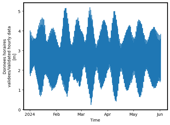
load and inspect tide gauge data

prod = False

tg = xr.open_dataset("data/94_2024.nc")
tg = tg.rename(Source4="sea level", TIME="time")

# extract lon/lat
lon_tg, lat_tg = float(tg.LONGITUDE), float(tg.LATITUDE)

# area of interest
extent = [-3, -1, 43.2, 44.5]
plot_map = lambda: pin.maps.plot_map(extent=extent, land=True, coastline=False)

# time = pd.date_range(start="2023/03/01", end="2023/08/01", freq="30T")
time = pd.to_datetime(tg.time)

tg["sea level"].plot()

[<matplotlib.lines.Line2D at 0x13d548f40>]

---

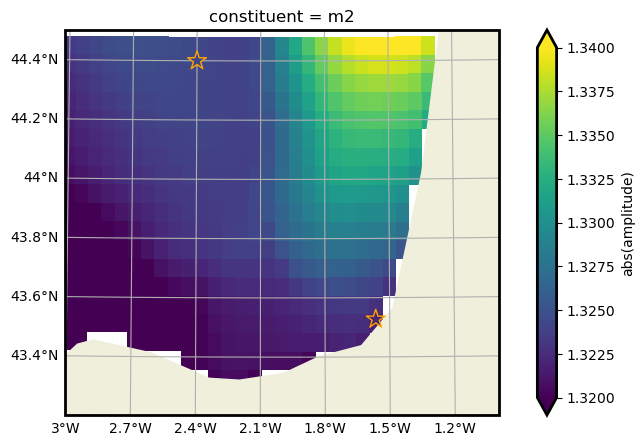
harmonic amplitudes in the area of interest

# positions of interest
moorings = dict(
    bayonne=[lon_tg - 0.05, lat_tg],  # offset tide gauge to be in water
    offshore=[-2.4, 44.4],
)
mo = (
    pd.DataFrame(moorings)
    .T.rename(columns={0: "lon", 1: "lat"})
    .to_xarray()
    .rename(index="mooring")
)

# output 2d grid
dl_min = 0.0625  # potential resolution: 0.0625
lon, lat = (extent[0], extent[1], dl_min), (extent[2], extent[3], dl_min)  # cp area

# load sea level and semi-diurnal constituents only
vtype = "z"
csts = td.major_semidiurnal
ds_2d = td.load_tidal_amplitudes(lon, lat, vtype, constituents=csts)
ds_moorings = td.load_tidal_amplitudes(mo.lon, mo.lat, vtype, constituents=csts)

broadcasting lon/lat

vmin = 1.32
vmax = 1.34

c = "m2"

# fig, ax = plot_map()
fig, ax, _ = plot_map()

_ds = ds_2d.sel(constituent=c)
(
    np.abs(_ds[vtype + "_amplitude"])
    .rename("abs(amplitude)")
    .plot(
        x="lon",
        y="lat",
        vmin=vmin,
        vmax=vmax,
        ax=ax,
        transform=crs,
    )
)

_ds = ds_moorings.sel(constituent=c)
h = ax.scatter(
    _ds.lon,
    _ds.lat,
    c=np.abs(_ds[vtype + "_amplitude"]),
    s=200,
    edgecolors="orange",
    marker="*",
    # _ds.lon, _ds.lat, c="w", s=100, edgecolors="0.5",
    vmin=vmin,
    vmax=vmax,
    transform=crs,
    zorder=10,
)

# load on FES grid - needs update
# ds = td.load_raw_tidal_amplitudes(["z", "u", "v"], lon=lon, lat=lat, constituents=td.major_semidiurnal)
# ds.sea_level_phase.sel(constituents="m2").plot()
# np.real(ds.sea_level_amplitude*np.exp(1j*ds.sea_level_phase*np.pi/180)).sel(constituents="m2").plot()

store all tidal harmonics

# prod = True
prod = False

nc = "bayonne_mooring_harmonics.nc"
if prod:
    ha = td.load_raw_tidal_amplitudes(["z", "u", "v"], lon=lon, lat=lat)
    ha.to_netcdf(nc, mode="w")
else:
    ha = xr.open_dataset(nc)

---

tidal predictions

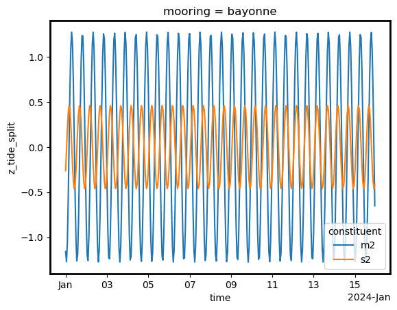
just sea level and (m2, s2)

# just m2 and s2
ds = td.tidal_prediction(
    mo.lon,
    mo.lat,
    time,
    [
        "z",
    ],
    constituents=td.major_semidiurnal,
    minor=False,
    split=True,
)
ds

<xarray.Dataset> Size: 206kB
Dimensions:       (mooring: 2, time: 3672, constituent: 2)
Coordinates:
  * mooring       (mooring) object 16B 'bayonne' 'offshore'
  * constituent   (constituent) object 16B 'm2' 's2'
    amplitude     (constituent) float64 16B 0.2441 0.1127
    phase         (constituent) float64 16B 1.732 0.0
    omega         (constituent) float64 16B 0.0001405 0.0001454
    alpha         (constituent) float64 16B 0.693 0.693
    species       (constituent) float64 16B 2.0 2.0
    omega_cpd     (constituent) float64 16B 1.932 2.0
  * time          (time) datetime64[ns] 29kB 2024-01-01 ... 2024-06-01T23:00:00
Data variables:
    lon           (mooring) float64 16B -1.565 -2.4
    lat           (mooring) float64 16B 43.53 44.4
    z_tide        (mooring, time) float64 59kB -1.423 -1.311 ... 0.6056 0.8539
    z_tide_split  (mooring, constituent, time) float64 118kB -1.16 ... -0.419

xarray.Dataset

• Dimensions:
  • mooring: 2
  • time: 3672
  • constituent: 2
• Coordinates: (9)
  • mooring
    (mooring)
    object
    'bayonne' 'offshore'

    array(['bayonne', 'offshore'], dtype=object)

  • constituent
    (constituent)
    object
    'm2' 's2'

    array(['m2', 's2'], dtype=object)

  • amplitude
    (constituent)
    float64
    0.2441 0.1127

    array([0.2441  , 0.112743])

  • phase
    (constituent)
    float64
    1.732 0.0

    array([1.73155755, 0.        ])

  • omega
    (constituent)
    float64
    0.0001405 0.0001454

    array([0.00014052, 0.00014544])

  • alpha
    (constituent)
    float64
    0.693 0.693

    array([0.693, 0.693])

  • species
    (constituent)
    float64
    2.0 2.0

    array([2., 2.])

  • omega_cpd
    (constituent)
    float64
    1.932 2.0

    array([1.93227358, 1.99999994])

  • time
    (time)
    datetime64[ns]
    2024-01-01 ... 2024-06-01T23:00:00

    array(['2024-01-01T00:00:00.000000000', '2024-01-01T01:00:00.000000000',
           '2024-01-01T02:00:00.000000000', ..., '2024-06-01T21:00:00.000000000',
           '2024-06-01T22:00:00.000000000', '2024-06-01T23:00:00.000000000'],
          dtype='datetime64[ns]')

• Data variables: (4)
  • lon
    (mooring)
    float64
    -1.565 -2.4

    array([-1.56482999, -2.4       ])

  • lat
    (mooring)
    float64
    43.53 44.4

    array([43.52732086, 44.4       ])

  • z_tide
    (mooring, time)
    float64
    -1.423 -1.311 ... 0.6056 0.8539

    array([[-1.42281391, -1.31060604, -0.86944291, ...,  0.2251058 ,
             0.6126459 ,  0.85475112],
           [-1.42099905, -1.3173044 , -0.8829164 , ...,  0.21354177,
             0.60555744,  0.85391592]])

  • z_tide_split
    (mooring, constituent, time)
    float64
    -1.16 -1.273 ... -0.4601 -0.419

    array([[[-1.16021138, -1.27292741, -1.06678413, ...,  0.60458946,
              1.07258966,  1.27191341],
            [-0.26260253, -0.03767864,  0.19734122, ..., -0.37948366,
             -0.45994375, -0.41716229]],
    
           [[-1.15535121, -1.27617851, -1.07733212, ...,  0.59140556,
              1.065621  ,  1.2729056 ],
            [-0.26564784, -0.04112589,  0.19441572, ..., -0.37786379,
             -0.46006356, -0.41898967]]])

• Indexes: (3)
  • mooring
    PandasIndex

    PandasIndex(Index(['bayonne', 'offshore'], dtype='object', name='mooring'))

  • constituent
    PandasIndex

    PandasIndex(Index(['m2', 's2'], dtype='object', name='constituent'))

  • time
    PandasIndex

    PandasIndex(DatetimeIndex(['2024-01-01 00:00:00', '2024-01-01 01:00:00',
                   '2024-01-01 02:00:00', '2024-01-01 03:00:00',
                   '2024-01-01 04:00:00', '2024-01-01 05:00:00',
                   '2024-01-01 06:00:00', '2024-01-01 07:00:00',
                   '2024-01-01 08:00:00', '2024-01-01 09:00:00',
                   ...
                   '2024-06-01 14:00:00', '2024-06-01 15:00:00',
                   '2024-06-01 16:00:00', '2024-06-01 17:00:00',
                   '2024-06-01 18:00:00', '2024-06-01 19:00:00',
                   '2024-06-01 20:00:00', '2024-06-01 21:00:00',
                   '2024-06-01 22:00:00', '2024-06-01 23:00:00'],
                  dtype='datetime64[ns]', name='time', length=3672, freq=None))

• Attributes: (0)

individual constituent contributions

tlim = ("2024/01/01", "2024/01/15")
da = ds["z_tide_split"].sel(mooring="bayonne", time=slice(*tlim))
da.plot.line(hue="constituent")

[<matplotlib.lines.Line2D at 0x15af81ae0>,
 <matplotlib.lines.Line2D at 0x15af364d0>]

total sea level prediction

# prod = True
prod = False

# with full list of harmonics
nc = "bayonne_moorings_time_series.nc"
if prod:
    tp = td.tidal_prediction(mo.lon, mo.lat, time, split=True)
    tp.to_netcdf(nc, mode="w")
else:
    tp = xr.open_dataset(nc)

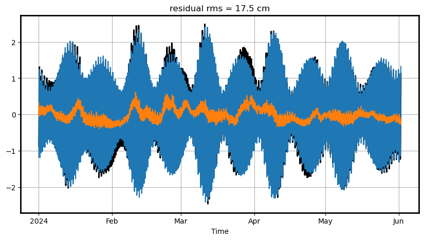
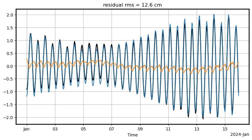
def plot_tseries(tg, tp, tlim=None):

    fig, ax = plt.subplots(1, 1, figsize=(10, 5))

    da = tg["sea level"]
    if tlim is not None:
        da = da.sel(time=slice(*tlim))
    da = da - da.mean("time")
    da.plot(color="k", lw=2)
    da_tg = da

    da = tp["z_tide"].sel(mooring="bayonne")
    if tlim is not None:
        da = da.sel(time=slice(*tlim))
    da.plot(hue="mooring")

    # ds["z_tide_minor"].sel(mooring="bayonne").plot()

    residual = da_tg - da
    residual.plot(label="residual")
    residual_rms = residual.std()

    ax.set_title(f"residual rms = {residual_rms*1e2:.1f} cm")

    ax.grid()

plot_tseries(tg, tp)
plot_tseries(tg, tp, tlim=("2024/01/01", "2024/01/15"))

---

misc: constituents, frequencies, equilibrium tides

td.cproperties

	amplitude	phase	omega	alpha	species	omega_cpd
constituent
m3	0.000000	0.000000	0.000000e+00	0.000	0.0	0.000000
eps2	0.000000	0.000000	0.000000e+00	0.000	0.0	0.000000
n4	0.000000	0.000000	0.000000e+00	0.000	0.0	0.000000
mtm	0.000000	0.000000	0.000000e+00	0.000	0.0	0.000000
msqm	0.000000	0.000000	0.000000e+00	0.000	0.0	0.000000
lambda2	0.000000	0.000000	0.000000e+00	0.000	0.0	0.000000
mks2	0.000000	0.000000	0.000000e+00	0.000	0.0	0.000000
r2	0.000000	0.000000	0.000000e+00	0.000	0.0	0.000000
s4	0.000000	0.000000	0.000000e+00	0.000	0.0	0.000000
s1	0.000000	0.000000	0.000000e+00	0.000	0.0	0.000000
sa	0.003104	6.232787	1.990970e-07	0.693	0.0	0.002738
ssa	0.019567	3.487600	3.982000e-07	0.693	0.0	0.005476
mm	0.022191	1.964022	2.639200e-06	0.693	0.0	0.036292
msf	0.003681	4.551628	4.925200e-06	0.693	0.0	0.067726
mf	0.042041	1.756042	5.323400e-06	0.693	0.0	0.073202
q1	0.019273	5.877718	6.495854e-05	0.695	1.0	0.893244
o1	0.100661	1.558554	6.759774e-05	0.695	1.0	0.929536
p1	0.046848	6.110182	7.252295e-05	0.706	1.0	0.997262
k1	0.141565	0.173004	7.292117e-05	0.736	1.0	1.002738
j1	0.007915	2.137025	7.556036e-05	0.695	1.0	1.039030
2n2	0.006141	4.086700	1.352405e-04	0.693	2.0	1.859690
mu2	0.007408	3.463115	1.355937e-04	0.693	2.0	1.864547
n2	0.046397	6.050721	1.378797e-04	0.693	2.0	1.895982
nu2	0.008811	5.427137	1.382329e-04	0.693	2.0	1.900839
m2	0.244100	1.731558	1.405189e-04	0.693	2.0	1.932274
l2	0.006931	0.553987	1.431581e-04	0.693	2.0	1.968565
t2	0.006608	0.052842	1.452450e-04	0.693	2.0	1.997262
s2	0.112743	0.000000	1.454441e-04	0.693	2.0	2.000000
k2	0.030684	3.487600	1.458423e-04	0.693	2.0	2.005476
mn4	0.000000	1.499093	2.783984e-04	0.693	0.0	3.828253
m4	0.000000	3.463115	2.810377e-04	0.693	0.0	3.864546
ms4	0.000000	1.731558	2.859630e-04	0.693	0.0	3.932274
m6	0.000000	5.194673	4.215566e-04	0.693	0.0	5.796819
m8	0.000000	6.926230	5.620755e-04	0.693	0.0	7.729093

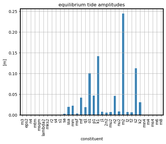
ax = td.cproperties.amplitude.plot.bar()
ax.set_title("equilibrium tide amplitudes")
ax.set_ylabel("[m]")
ax.grid()

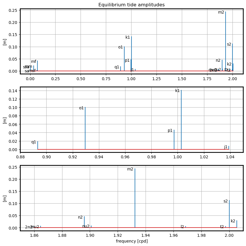
fig, axes = plt.subplots(3, 1, figsize=(10, 10))
td.plot_equilibrium_amplitudes(td.cproperties, axes[0])
td.plot_equilibrium_amplitudes(td.cproperties, ax=axes[1], xlim=(0.88, 1.05))
td.plot_equilibrium_amplitudes(td.cproperties, ax=axes[2], xlim=(1.85, 2.01))

for i in range(0, 2):
    axes[i].set_xlabel("")
for i in range(1, 3):
    axes[i].set_title("")

play with tidal arguments used for predictions

$ \begin{align} \eta = \mathcal{R} \Big { \sum_k h_k \times f_k(t) h_c e^{i (g_k(t) + u_k(t) ) } \Big } \end{align} $

$g_k (t)$ is the equilibrium argument, it is common to all models $f_l(t)$ and $u_k(t)$ are nodal corrections.

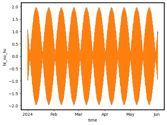
Constituents have unit complex amplitudes here:

ds = td.get_tidal_arguments(time)

_ds = ds
# _ds = ds.isel(time=slice(0,24*28))
np.real(_ds["ht_no_hc"]).sel(constituent=td.major_semidiurnal).sum("constituent").plot()
np.imag(_ds["ht_no_hc"]).sel(constituent=td.major_semidiurnal).sum("constituent").plot()

[<matplotlib.lines.Line2D at 0x14375ea70>]