Timeseries module - demo#
pynsitu.tseries implements methods useful to the time series analysis
Assumptions about the data
import xarray as xr
import pandas as pd
import numpy as np

import matplotlib.pyplot as plt

import pynsitu as pin
Warning: could not import pytide
generate synthetic time series#
tdefault = dict(start="2018-01-01", end="2018-01-30", freq="1h")


def generate_time_series(label="time", uniform=True, time_units="datetime"):
    """Create a drifter time series."""
    time = pd.date_range(**tdefault)
    time_scale = pd.Timedelta("1D")
    if time_units == "timedelta":
        time = time - time[0]
    elif time_units == "numeric":
        time = (time - time[0]) / pd.Timedelta("1h")
        time_scale = 1.0
    if not uniform:
        nt = time.size
        import random

        random.seed(1001)
        time = time[random.sample(range(nt), 2 * nt // 3)].sort_values()
    #
    rng = np.random.default_rng(12345)
    v0 = (
        np.cos(2 * np.pi * ((time - time[0]) / time_scale))
        + rng.normal(size=time.size) / 2
    )
    v1 = (
        np.sin(2 * np.pi * ((time - time[0]) / time_scale))
        + rng.normal(size=time.size) / 2
    )
    df = pd.DataFrame({"v0": v0, "v1": v1, label: time})
    df = df.set_index(label)
    return df
# actually generate one time series
df = generate_time_series(uniform=False)
df.head()
| v0 | v1 | |
|---|---|---|
| time | ||
| 2018-01-01 02:00:00 | 0.288087 | 0.554390 |
| 2018-01-01 03:00:00 | 1.597790 | -0.565405 |
| 2018-01-01 05:00:00 | 0.271776 | 0.536564 |
| 2018-01-01 07:00:00 | 0.129232 | 0.903828 |
| 2018-01-01 09:00:00 | -0.296491 | 1.024384 |
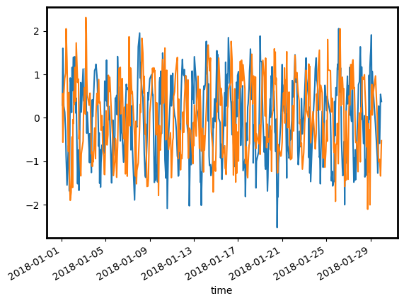
df.v0.plot()
df.v1.plot();
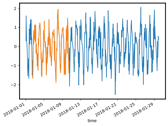
basic editing#
triming based on deployment information#
d = pin.events.Deployment(
    "some_event",
    start="2018/01/02 12:12:00",
    end="2018/01/10 12:12:00",
)

df_trimmed = df.ts.trim(d)

df.v0.plot()
df_trimmed.v0.plot()
<Axes: xlabel='time'>
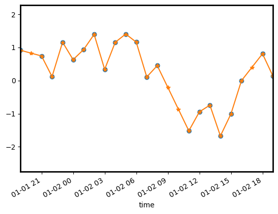
resampling on a regular timeline#
df_resampled = df.ts.resample_uniform("1h")
fig, ax = plt.subplots(1, 1)
df.v0.plot(marker="o", ls="None")
df_resampled.v0.plot(marker="*")
ax.set_xlim(df.index[10], df.index[30])
(np.float64(17532.791666666668), np.float64(17533.791666666668))
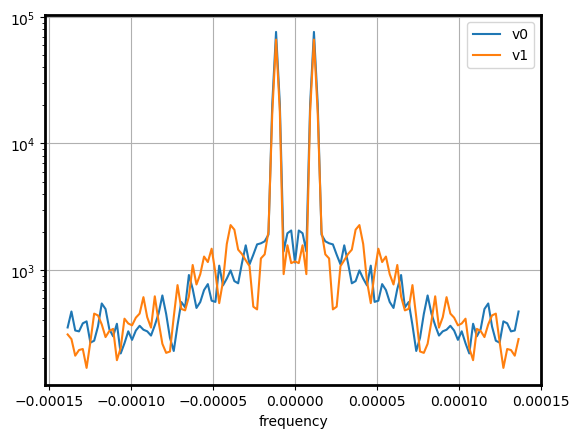
spectral analysis#
E = df_resampled.ts.spectrum(nperseg=24 * 5)
E
| v0 | v1 | |
|---|---|---|
| frequency | ||
| -0.000139 | 351.074214 | 309.222013 |
| -0.000137 | 469.446684 | 284.267359 |
| -0.000134 | 332.358004 | 210.038744 |
| -0.000132 | 326.892586 | 232.814772 |
| -0.000130 | 378.643108 | 237.213704 |
| ... | ... | ... |
| 0.000127 | 392.326265 | 168.116599 |
| 0.000130 | 378.643108 | 237.213704 |
| 0.000132 | 326.892586 | 232.814772 |
| 0.000134 | 332.358004 | 210.038744 |
| 0.000137 | 469.446684 | 284.267359 |
120 rows × 2 columns
E.plot()
plt.yscale("log")
plt.grid()
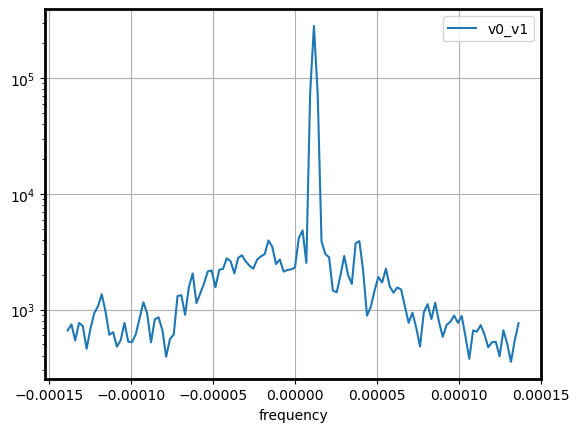
rotary spectrum#
Compute the spectrum of v0 + 1j v1
E = df_resampled.ts.spectrum(nperseg=24 * 5, complex=("v0", "v1"))
E.plot()
plt.yscale("log")
plt.grid()
filtering#
to be done …
tidal analysis#
to be done …
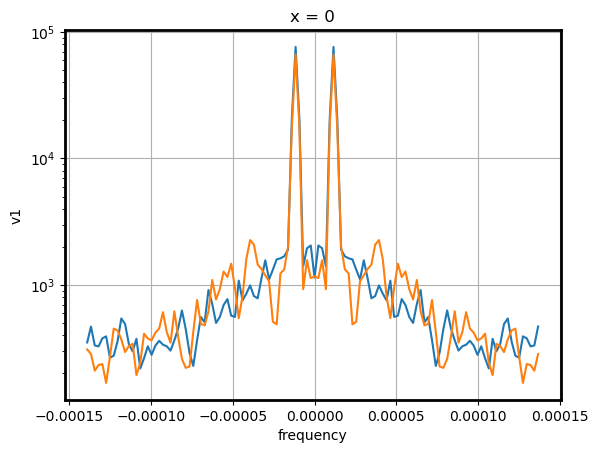
with xarray objects#
ds = df_resampled.to_xarray().expand_dims(x=range(10)).chunk(dict(x=2))
ds
<xarray.Dataset> Size: 117kB
Dimensions:  (x: 10, time: 695)
Coordinates:
  * x        (x) int64 80B 0 1 2 3 4 5 6 7 8 9
  * time     (time) datetime64[ns] 6kB 2018-01-01T02:00:00 ... 2018-01-30
Data variables:
    v0       (x, time) float64 56kB dask.array<chunksize=(2, 695), meta=np.ndarray>
v1 (x, time) float64 56kB dask.array<chunksize=(2, 695), meta=np.ndarray>E = ds.ts.spectrum(nperseg=24 * 5)
E.v0.isel(x=0).plot()
E.v1.isel(x=0).plot()
plt.yscale("log")
plt.grid()
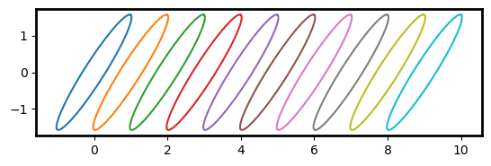
vector principal axes/ellipse#
def compute_vector_principal_axes(u, v):
    """Compute vector time series principal axes
    See Emery and Thomson section 4.4.1

    Parameters
    ----------
        u, v: xr.DataArray
        Must possess `time` dimension

    Returns
    -------
        major, minor: xr.DataArray
        Complex arrays corresponding to major/minor axes scaled by respective eigenvalues
        The orientation of each axis is thus provided by the complex angle
    """

    # demean
    u_mean, v_mean = u.mean("time"), v.mean("time")
    up = u - u_mean
    vp = v - v_mean

    # build velocity covariance array and return eigenvectors
    uu = (up * up).mean("time")
    uv = (up * vp).mean("time")
    vv = (vp * vp).mean("time")

    # proceed with principal axes calculation  see Emery and Thomson 4.53
    ke = (uu + vv) * 0.5
    det = np.sqrt((uu - vv) ** 2 + 4 * uv**2)
    lambda_1 = ke + det * 0.5
    lambda_2 = ke - det * 0.5
    #
    s_1 = (lambda_1 - uu) / uv
    e_1 = (1 + 1j * s_1) / np.sqrt(1 + s_1**2)
    # compute vectors scaled by eigenvalues
    major = lambda_1 * e_1
    minor = lambda_2 * e_1 * np.exp(1j * np.pi / 2)

    return major, minor


def build_principal_ellipse(major, minor, scale=1):
    """build principal ellipse for drawing purposes"""
    # build ellipse
    t = xr.DataArray(np.linspace(0, 2 * np.pi, 100), dims="time").rename("time")
    v = (np.cos(t) * major + np.sin(t) * minor) * scale
    x = np.real(v)
    y = np.imag(v)
    return x, y
u = ds.v0
v = ds.v0 + ds.v1  # introduces correlation to rotate the ellipse
v_major, v_minor = compute_vector_principal_axes(u, v)

# check variances is preserved:
float(np.abs(v_major).compute()[0]) + float(np.abs(v_minor).compute()[0]), float(
    (u.std("time") ** 2 + v.std("time") ** 2).compute()[0]
)
(2.1267873595224254, 2.126787359522425)
# plot
x, y = build_principal_ellipse(v_major, v_minor)

fig, ax = plt.subplots(1, 1)
ax.plot(x + x.x, y)
ax.set_aspect("equal")